Stereo Vision for Obstacle and Lane Detection
This project implements a pipeline for obstacle and lane marking detection from stereo camera input, using traditional computer vision techniques such as disparity estimation, edge detection, and Hough transforms.
Project Goals
Detect lane markings and obstacles using stereo vision, disparity maps, and geometric reasoning — without deep learning.
Input stereo images
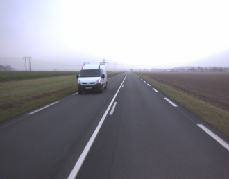
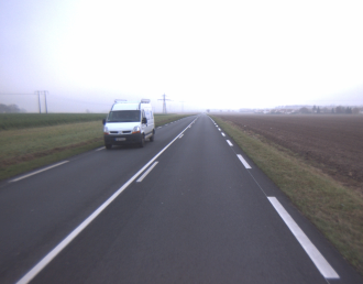
Initial stereo image pair (left and right views).
Main Processing steps
- Applied morphological filtering and edge detection to extract structural features.
- Lane markings were further isolated by subtracting a low-pass filtered version of the image (using a rectangular median local threshold filter), which enhanced horizontal high-frequency components. This helped distinguish lane markings from vehicles or other low-frequency features.
- Constructed a vertical disparity map (
v-disparity) to identify the road plane and detect vertical features above it. - Applied Hough transform in v-disparity space to extract dominant straight lines.
- Two key lines in this space represent the set of lane boundaries and the elevated structure (i.e., the vehicle in our scene).
- Compared multiple filtering strategies (mean, median, morphological opening, and Canny edge detection) to assess their relative performance in lane and obstacle extraction.
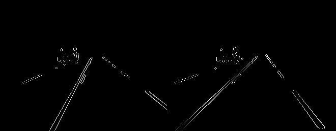

Detected edges, v-disparity map, and Hough line detection.
Road Profile Estimation
We used the vertical disparity map (v-disparity) to model the road surface.
The bottom part of the v-disparity image shows a linear pattern corresponding to the ground plane.
A Hough transform was applied in the v-disparity space to detect this line.
Points significantly above this line were flagged as potential vertical obstacles.
The horizontal position (u) and vertical (v) disparity together reconstruct the 3D geometry of the scene.
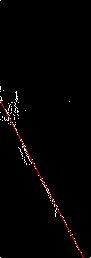

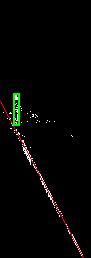
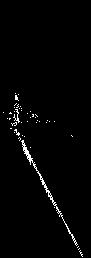
Left: set of lane markings; Middle: closest obstacle; Right: colored v-disparity map.
Evaluation and Thresholding Analysis
To evaluate the performance of lane marking detection, we varied the binarization threshold. We plotted the detection rate and false alarm rate as the threshold varies.
A tighter threshold detects more pixels of lane markings but increases false positives; a looser threshold reduces false alarms but may miss target pixels.
Colored disparity map
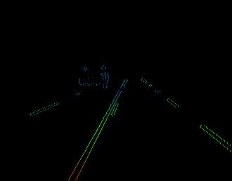
Pixel color: red -> blue corresponds to near -> far depth.
Final results
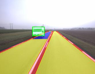
Scene segmentation: red = lane markings, yellow = road, blue = occupied area, green = detected obstacle.
Tools Used
- Matlab: implemented the entire detection pipeline using image processing toolbox and custom stereo geometry code.